고정 헤더 영역
상세 컨텐츠
본문
Turning any CNN image classifier into an object detector with Keras, TensorFlow, and OpenCV - PyImageSearch
In this tutorial, you will learn how to take any pre-trained deep learning image classifier and turn it into an object detector using Keras, TensorFlow, and OpenCV.
www.pyimagesearch.com
Turning CNN into Object Detectors
1. Fundamentals of object detection
Things you will learn:
- image pyramids,
- sliding windows,
- non-maxima suppression (HOG + SVM inspired)
2. Image Classification vs Object Detection

Image Classification:
- 입력: 이미지 하나 / 출력: 클레스 레이블 하나
Object Detection
- 입력: 이미지 하나 / 출력: 다수의 (1) 이미지에 무엇이 들어가 있는지 (2) 그것이 어디에 있는지
Object Detection 의 기본적인 구조
- 입력: 객체 탐지를 할 이미지
- 출력:
- bounding boxes (각 객체에 대한 x, y 좌표)
- class labels (각 객체에 대한)
- probability/confidence score (각 박스와 레이블에 대한)
3. Image Classifier → Object Detector
이미 이미지 분류를 한 CNN 모델이 있는데, 이걸 어떻게 객체 탐지 모델로 바꿀 수 있나요?
객체 탐지 모델은 분류 모델보다 더 복잡한 구조를 가짐. But 전통적인 컴퓨터 비전 알고리즘에 해답이 있음
딥러닝 기반 객체 탐지 이전에 가장 최신 기술은 HOG + Linear SVM이었음. 이 방식의 요소들을 빌려와서 모델을 변환해보겠음.
첫번째 요소:
- Image Pyramids: A multi-scale representation of an image

위와 같은 피라미드 형태의 다층 구조는 객체를 다양한 사이즈(스케일)로 탐지할 수 있게끔 함
- 가장 밑바닥에는 원본 사이즈(가로 * 높이)의 원본 이미지가 있음.
- 위 레이어로 올라갈 때마다, 이미지는 resize (subsampled)됨. (선택적으로 가우시안 블러링을 통해 smooth되기도 함)
- 특정 조건을 만족하기 이전까지는 레이어 위로 올라감. (일반적으로 추가적인 subsampling이 필요 없는 최소 사이즈에 도달했을 경우임)
두번째 요소:
- Sliding Windows: 고정된 크기의 직사각형(window)이 좌측 상단에서부터 우측 하단까지 훑는 것

탐색하면서 다음과 같은 동작을 실시함:
- ROI 추출 (Regions of Interest)
- 이미지 분류기(Linear SVM, CNN 등)에 통과
- 출력 예측값을 획득
Image pyramid & Sliding window = 객체를 다른 위치에서 각기 다른 크기로 localize할 수 있게 함
세번째 요소:
- Non-Maxima Suppression (NMS): 객체 탐지를 할 때 일반적으로 다수의 겹치는 bounding boxes를 만드는데, 그 중 confidence(신뢰도)가 낮은 박스를 suppress(억제)하여, 가장 신뢰도가 높은 박스를 남기게 하는 방식.

다수의 박스는 애초에 문제점을 가지고 있음. 이미지에는 하나의 물체만 있는데, 다수의 박스를 반환하는 것은 말도 안 됨. 그래서 신뢰도가 낮은 것은 없애고 가장 신뢰도가 높은 것은 남기는 과정을 거쳐야 함.
전통적인 컴퓨터 비전 방식을 통해 이미지 분류기를 객체 탐지로 바꾸는 일련의 과정은 다음과 같이 정리:

실습해보자
파일구조는 다음과 같음:

detection_helpers.py에는 다음과 같은 함수가 들어있음:
- image_pyramid: 다양한 크기의 이미지로 객체를 탐지할 수 있도록 이미지를 다양한 크기로 복사해줌
- sliding_window: 객체가 어디에 있는지 알려줌. 분류 window를 좌에서 우로, 위에서 아래로 이동시킴.
detection_helpers.py 파일의 도움을 받아서 detect_with_classifier.py 는 이미지 분류에서 객체 탐지로 방식을 바꿀 수 있음. 우리가 사용할 분류기는 이미지넷 데이터셋을 학습한 ResNet50 컨볼루션 모델임. 위 세 가지 종류의 이미지는 테스트할 목적으로 제공됨.
첫번째 함수 구현:

3가지 파라이터를 받는 제너레이터 함수임:
- image: window를 반복적으로 탐색시킬 입력 이미지. (image pyramid의 결과물을 활용해도 됨)
- step: x, y의 방향으로 몇 픽셀만큼 skip 할건지 지정. 1이면 모든 픽셀을 탐지하는 것이므로 부적합하고, 일반적으로 4, 8 정도가 적당함. 숫자가 작을 수록 검토해야 하는 window가 많아짐
- ws: window size의 약자. window의 (픽셀단위) 가로와 높이.
실질적인 window의 "sliding"은 (6-9)에서 실시된다. 위 함수는 이중 for문으로 이루어져있는데, 각각 행 기준, 열 기준임. return 대신에 yield를 사용했기 때문에 이 함수는 제너레이터임.
두번째 함수 구현:

두번째 함수 역시 3가지 파라미터를 받음:
- image: 우리가 다중 스케일을 제너레이트하고 싶은 입력 이미지 (즉, 피라미트 만들고 싶은 대상)
- scale: 각 레이어마다 resize되는 scale factor. 값이 작을수록 더 많은 층을 만들고, 값이 클수록 더 작은 층을 만듦
- minSize: 피라미트 층의 출력 이미지의 최소 사이즈를 조절. 이 기준점이 없으면 피라미드에서 무한정하게 이미지를 축소시켜나가면서 제너레이트함. (그러면 안 되겠죠?)
image_pyramid에서 첫번째로 생성되는 이미지는 원본 사이즈의 이미지임. (13) 위에 있는 모나리자 그림 피라미드(Figure 2)를 보면 가장 아래층에 원본 이미지가 있는 부분임.
while True 반복문으로 무한정 반복이 실시됨. (16) 주어진 scale 값에 따라 다음 레이어의 크기를 계산하는데, 우리의 코드 같은 경우 단순하게 이미지의 폭을 scale로 나눠서 w 비율값을 결정하게 함. (18) 그 다음 이미지를 imutils.resize하게 됨. (19) 이미지 크기 조정 이후 주어진 minSize 값에 의하여 이미지가 너무 작다면 반복문을 탈출하게 됨. (23-24) minSize 기준을 통과했다면 피라미드의 다음 이미지를 만들어 냄. (27)
코드 정리:
더보기
# detection_helpers.py
# import the necessary packages
import imutils

def sliding_window(image, step, ws):
	# slide a window across the image
	for y in range(0, image.shape[0] - ws[1], step):
		for x in range(0, image.shape[1] - ws[0], step):
			# yield the current window
			yield (x, y, image[y:y + ws[1], x:x + ws[0]])

def image_pyramid(image, scale=1.5, minSize=(224, 224)):
	# yield the original image
	yield image

	# keep looping over the image pyramid
	while True:
		# compute the dimensions of the next image in the pyramid
		w = int(image.shape[1] / scale)
		image = imutils.resize(image, width=w)

		# if the resized image does not meet the supplied minimum
		# size, then stop constructing the pyramid
		if image.shape[0] < minSize[1] or image.shape[1] < minSize[0]:
			break

		# yield the next image in the pyramid
		yield image
detect_with_classifier.py는 다음과 같음:
1) 먼저 필요한 라이브러리를 임포트함 (1-13)

2) 다음으로는 argument parsing: (16-25)

따라서, 터미널에서 파이썬 파일을 실행시킬 때 다음과 같은 argument가 요구됨:
- --image: 객체 탐지를 할 이미지의 경로
- --size: 튜플, sliding window의 크기. 쌍따옴표로 둘러싸야 함 (e.g. "(200, 150)")
- --min-cof: bounding boxes를 걸러줄 최소 신뢰도 값
- --visualize: 디버깅을 위해 추가적으로 시각화를 해줄지 여부
3) 다음은 몇 가지 constants 정의: (28-32)

- WIDTH: 각 이미지가 같은 사이즈가 아니기 때문에 시작할 때의 사이즈는 일정하도록 고정시킴
- PYR_SCALE: image_pyramid 함수의 scale factor. 각 층마다 어느 비율로 크기가 조정되는지 나타냄. 값이 작을수록 더 많은 층이 생기고, 값이 클수록 적은 층이 생김. 층이 더 적을 수록 전반적인 객체 탐지 과정은 빠르게 작동하지만, 정확도는 떨어질 수도 있음
- WIN_STEP: sliding window 가 x, y 방향으로 skip하는 픽셀의 값. 이 값이 작을수록 더 많은 windows를 검토해야 하고 더 느려짐. 실질적으로 4 혹은 8 정도의 값이 적당함. (입력 이미지의 크기나 minSize의 값에 따라서 좀 다르긴 함)
- ROI_SIZE: 탐지하고 싶은 객체의 크기 비율을 조절함. 만약에 이 비율에서 문제가 있으면 객체를 탐지하는 건 거의 불가능임. 추가적으로 이 값은 minSize 값과 연관이 되어있음. (minSize는 반복문에서 탈출하는 것을 결정한다는 걸 기억할 것) ROI_SIZE는 cmd에 주어질 argument 중 --size와 직접적으로 연관됨.
- INPUT_SIZE: CNN 분류기의 차원 크기. 이 값은 당신이 사용할 CNN에 따라서 크게 달라질 수 있음. (우리의 경우 ResNet50를 사용함)
위 상수값들이 무엇을 조절하고 있는지 이해하는 것은 이미지 분류기를 객체 탐지기로 성공적으로 변환하는 데에 결정적임. 다음 내용을 알아보기 전에 반드시 위 내용을 숙지할 것.
ResNet 기반 CNN 분류기와 입력 이미지를 로드해보자.

이미지넷으로 사전훈련된 ResNet을 로드한다. (36) 당면한 문제에 따라 다른 사전 훈련된 모델을 고를 수도 있음.
또한, 인풋 이미지도 로드함. 로드된 후에는 resize한다. (가로세로 비율은 유지함) (40-41)
이제 image pyramid generator 객체를 초기화한다.

image_pyramid 함수에 필요한 파라미터를 공급하자. pyramid가 생성자 객체이기 때문에 우리는 반복적으로 값을 생성할 수 있다. 반복적으로 생성하기 전에 두 개의 빈 리스트를 만든다:
- rois: pyramid와 sliding window의 출력으로 만들어진 ROI를 담는다
- locs: ROI가 원래 이미지에 있었던 (x, y) 좌표를 담는다
또한 우리는 start라는 변수를 통해 시간이 얼마나 걸렸는지를 알 수 있다.
pyramid의 각 image를 반복하자.

반복문에서 먼저해야할 것은 원래 이미지 크기 (W)와 현재 레이어의 크기 (image.shape[1]) 사이의 scale factor를 계산하는 것이다. 이 값은 나중에 객체 bounding boxes를 upscale하는 데 사용될 것이다.
다음으로, 현재 머물러 있는 image pyramid의 레이어에서 sliding window 반복문으로 들어가보자. slinding_window 생성자가 만들어낸 각 ROI마다 우리는 이미지 분류를 적용할 것이다.
sliding window 반복문 내에서 다음과 같이 실시한다:
- scale 좌표를 구하고
- ROI를 전처리한다. 전처리는 resize, 배열 형식으로 변환, 케라스의 전처리 함수를 적용하는 것이다. 전처리 함수에는
- batch dimension을 추가하는 것,
- RGB를 BGR로 변환하는 것,
- 이미지넷 데이터셋에 따라 color 채널을 zero-center하는 것을 포함한다.
- rois와 locs 리스트를 업데이트한다.
선택적으로 시각화를 조절할 수 있다:
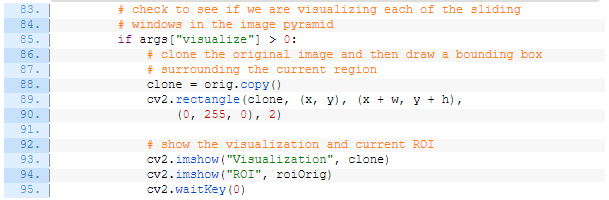
여기서 우리는 원본 이미지와 resize된 ROI에 초록색 박스를 그려 현재 어디를 "보고" 있는지를 시각화한다. 코드에서 보다시피, 우리는 터미널에서 --visualize 값이 설정되었을 때만 시각화한다.
다음으로 우리는
- pyramid + sliding window 과정이 어떻게 되어가고 있는지 확인하고 (check the benchmark)
- 모든 rois에 대해서 분류하고
- 예측값을 해석(decode)할 것이다.

먼저, end 변수에서 이 과정이 얼마나 오래 걸렸는지를 확인한다.
그리고 나서, 우리는 ROI를 가지고 사전학습된 이미지 분류기에 predict를 통해 각 배치 사이즈로 주입시킨다. 코드에서 볼 수 있다시피, 성능을 확인할 수 있는 지표를 출력해주고 있다.
마지막으로, 예측값을 해석하고 있는데, 각 ROI에서 가장 높은 예측값만 가져온다.
클래스 레이블 값(keys)과 ROI 좌표값(values)을 매핑시킬 딕셔너리 labels를 준비한다.
labels 딕셔너리를 채워넣도록 하자:
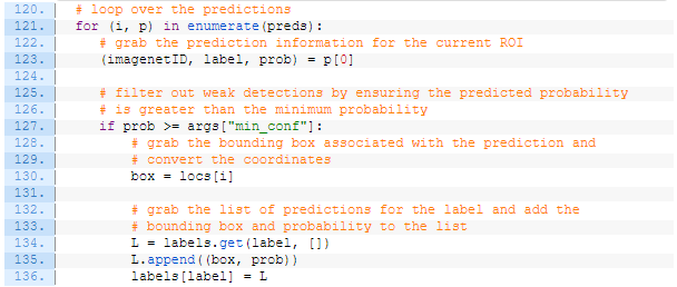
예측을 반복하여 현재 ROI에 대한 imagenetID, label, prob 값을 가져온다.
다음으로, prob이 최소 신뢰도 값을 넘었는지 확인한다. 이를 통과하였다면, labels 딕셔너리에 각 label(key 값)에 해당하는 box와 prob (신뢰도 값)을 업데이트 해준다.
현재까지 한 것을 정리해보자면, 우리는:
- image pyramid를 활용해 scaled된 이미지를 생성했고
- sliding window 접근법을 이용하여 image pyramid의 각 레이어(scaled image)에 대해 ROI를 생성했고
- 각 ROI에 대해서 분류를 실시하고 해당 결과를 labels 리스트에 업데이트했다
여태까지 한 것만으로 우리는 이미지 분류기를 객체 탐지기로 변환시켰다고 할 순 없다. 이제 우리는 이 결과를 시각화할 필요가 있다.
이제는 얻은 결과(labels)를 통해 무언가 유용한 것을 해야할 단계다. 이번 사례의 경우 우리는 단순히 객체에 레이블을 달아주도록 하겠다. 또한 우리는 겹치는 객체 탐지를 NMS를 통해 해결하도록 하겠다.
labels 리스트에 있는 모든 keys에 대해서 반복문을 실시해보자.

labels에 있는 각 탐지된 객체에 대해서 반복문을 돌린다. (139)
레이블링을 하기 위해 원본 이미지의 복사본을 만들자. (142)
그리고 나선 현재의 label에 대해서 모든 bounding boxes를 레이블링한다. (145-149)
NMS 적용 이전 vs 이후에 대해서 시각화를 하기 위해서 "Before"이미지를 보여주고 복사본을 만든다.
NMS 적용 이후를 보여주도록 하자:

NMS를 적용하기 위해서 우리는 bounding boxes와 그와 연관된 신뢰도를 추출한다. (159-160) 그리고 나선 그 결과들을 imutils에서 임포팅한 non_max_suppresion에 통과시켜준다. (161)
NMS가 적용된 이후에는 "After" bounding box 직사각형들에 레이블링을 해준다. (165-171) 이후 결과를 보여준다. (174-175)
코드 정리:
더보기
# import the necessary packages
from tensorflow.keras.applications import ResNet50
from tensorflow.keras.applications.resnet import preprocess_input
from tensorflow.keras.preprocessing.image import img_to_array
from tensorflow.keras.applications import imagenet_utils
from imutils.object_detection import non_max_suppression
from pyimagesearch.detection_helpers import sliding_window
from pyimagesearch.detection_helpers import image_pyramid
import numpy as np
import argparse
import imutils
import time
import cv2

# construct the argument parse and parse the arguments
ap = argparse.ArgumentParser()
ap.add_argument("-i", "--image", required=True,
	help="path to the input image")
ap.add_argument("-s", "--size", type=str, default="(200, 150)",
	help="ROI size (in pixels)")
ap.add_argument("-c", "--min-conf", type=float, default=0.9,
	help="minimum probability to filter weak detections")
ap.add_argument("-v", "--visualize", type=int, default=-1,
	help="whether or not to show extra visualizations for debugging")
args = vars(ap.parse_args())

# initialize variables used for the object detection procedure
WIDTH = 600
PYR_SCALE = 1.5
WIN_STEP = 16
ROI_SIZE = eval(args["size"])
INPUT_SIZE = (224, 224)

# load our network weights from disk
print("[INFO] loading network...")
model = ResNet50(weights="imagenet", include_top=True)

# load the input image from disk, resize it such that it has the
# has the supplied width, and then grab its dimensions
orig = cv2.imread(args["image"])
orig = imutils.resize(orig, width=WIDTH)
(H, W) = orig.shape[:2]

# initialize the image pyramid
pyramid = image_pyramid(orig, scale=PYR_SCALE, minSize=ROI_SIZE)

# initialize two lists, one to hold the ROIs generated from the image
# pyramid and sliding window, and another list used to store the
# (x, y)-coordinates of where the ROI was in the original image
rois = []
locs = []

# time how long it takes to loop over the image pyramid layers and
# sliding window locations
start = time.time()

# loop over the image pyramid
for image in pyramid:
	# determine the scale factor between the *original* image
	# dimensions and the *current* layer of the pyramid
	scale = W / float(image.shape[1])

	# for each layer of the image pyramid, loop over the sliding
	# window locations
	for (x, y, roiOrig) in sliding_window(image, WIN_STEP, ROI_SIZE):
		# scale the (x, y)-coordinates of the ROI with respect to the
		# *original* image dimensions
		x = int(x * scale)
		y = int(y * scale)
		w = int(ROI_SIZE[0] * scale)
		h = int(ROI_SIZE[1] * scale)

		# take the ROI and preprocess it so we can later classify
		# the region using Keras/TensorFlow
		roi = cv2.resize(roiOrig, INPUT_SIZE)
		roi = img_to_array(roi)
		roi = preprocess_input(roi)

		# update our list of ROIs and associated coordinates
		rois.append(roi)
		locs.append((x, y, x + w, y + h))

        # check to see if we are visualizing each of the sliding
		# windows in the image pyramid
		if args["visualize"] > 0:
			# clone the original image and then draw a bounding box
			# surrounding the current region
			clone = orig.copy()
			cv2.rectangle(clone, (x, y), (x + w, y + h),
				(0, 255, 0), 2)

			# show the visualization and current ROI
			cv2.imshow("Visualization", clone)
			cv2.imshow("ROI", roiOrig)
			cv2.waitKey(0)

# show how long it took to loop over the image pyramid layers and
# sliding window locations
end = time.time()
print("[INFO] looping over pyramid/windows took {:.5f} seconds".format(
	end - start))

# convert the ROIs to a NumPy array
rois = np.array(rois, dtype="float32")

# classify each of the proposal ROIs using ResNet and then show how
# long the classifications took
print("[INFO] classifying ROIs...")
start = time.time()
preds = model.predict(rois)
end = time.time()
print("[INFO] classifying ROIs took {:.5f} seconds".format(
	end - start))

# decode the predictions and initialize a dictionary which maps class
# labels (keys) to any ROIs associated with that label (values)
preds = imagenet_utils.decode_predictions(preds, top=1)
labels = {}

# loop over the predictions
for (i, p) in enumerate(preds):
	# grab the prediction information for the current ROI
	(imagenetID, label, prob) = p[0]

	# filter out weak detections by ensuring the predicted probability
	# is greater than the minimum probability
	if prob >= args["min_conf"]:
		# grab the bounding box associated with the prediction and
		# convert the coordinates
		box = locs[i]

		# grab the list of predictions for the label and add the
		# bounding box and probability to the list
		L = labels.get(label, [])
		L.append((box, prob))
		labels[label] = L

# loop over the labels for each of detected objects in the image
for label in labels.keys():
	# clone the original image so that we can draw on it
	print("[INFO] showing results for '{}'".format(label))
	clone = orig.copy()

	# loop over all bounding boxes for the current label
	for (box, prob) in labels[label]:
		# draw the bounding box on the image
		(startX, startY, endX, endY) = box
		cv2.rectangle(clone, (startX, startY), (endX, endY),
			(0, 255, 0), 2)

	# show the results *before* applying non-maxima suppression, then
	# clone the image again so we can display the results *after*
	# applying non-maxima suppression
	cv2.imshow("Before", clone)
	clone = orig.copy()

    # extract the bounding boxes and associated prediction
	# probabilities, then apply non-maxima suppression
	boxes = np.array([p[0] for p in labels[label]])
	proba = np.array([p[1] for p in labels[label]])
	boxes = non_max_suppression(boxes, proba)

	# loop over all bounding boxes that were kept after applying
	# non-maxima suppression
	for (startX, startY, endX, endY) in boxes:
		# draw the bounding box and label on the image
		cv2.rectangle(clone, (startX, startY), (endX, endY),
			(0, 255, 0), 2)
		y = startY - 10 if startY - 10 > 10 else startY + 10
		cv2.putText(clone, label, (startX, y),
			cv2.FONT_HERSHEY_SIMPLEX, 0.45, (0, 255, 0), 2)

	# show the output after apply non-maxima suppression
	cv2.imshow("After", clone)
	cv2.waitKey(0)
'Coding > Image' 카테고리의 다른 글
| [3] Region Proposal Object Detection (0) | 2021.04.12 |
|---|---|
| [2] Selective Search (0) | 2021.04.12 |
| matplot RGB vs opencv BGR vs caffe images (0) | 2021.04.09 |
| OpenCV fundamentals (0) | 2021.04.09 |
| Scene Text Recognition (0) | 2021.04.01 |


