고정 헤더 영역
상세 컨텐츠
본문
Object detection: Bounding box regression with Keras, TensorFlow, and Deep Learning - PyImageSearch
Object detection: Bounding box regression with Keras, TensorFlow, and Deep Learning - PyImageSearch
In this tutorial you will learn how to train a custom deep learning model to perform object detection via bounding box regression with Keras and TensorFlow.
www.pyimagesearch.com
2020년 10월 5일 포스팅
들어가며
이 튜토리얼에선 이미지 객체에 바운딩 박스를 그려주는 우리만의 맞춤형 딥러닝 모델을 만드는 방법에 대해서 알아보도록 하겠습니다.
이전 RCNN에 대한 4개의 글을 읽고 나면 "모델이 전체적으로 어떻게 구동되는지는 알겠는데, 바운딩 박스 회귀는 어떻게 되는지 잘 이해가 안 된다"는 분이 있으셔서 이 글을 작성하게 되었습니다.
기초적인 RCNN 객체 탐지 모델은 구역 제안(region proposal) 생성기라는 개념를 바탕으로 만들어집니다. 이러한 구역 제안 알고리즘은 (가령 Selective search 등) 입력 이미지를 살펴보고 잠재적으로 객체가 어디에 있을 것 같은지 알려줍니다. 주의할 점은 이 알고리즘은 제안된 특정 구역에 대해서 객체가 있을지 전혀 모른다는 것입니다. 이 알고리즘은 단순히 이미지에서 좀 더 살펴볼 가치가 있는 "흥미로운 구역"을 제안할 뿐입니다.
전형적인 RCNN 모델은 (1) 이 제안 구역을 사전 학습된 합성곱 신경망에 주입하여 특성(혹은 feature)을 출력하였고, (2) 그런 다음에 그 출력된 특성을 SVM에 주입하여 최종적인 분류를 실시하였습니다. 이러한 방식의 구현에서는 구역 제안 알고리즘이 제안하는 지점이 "바운딩 박스"로 취급되었고, SVM은 그 바운딩 박스에 대해서 클래스 레이블을 제공하는 역할을 했던 것입니다.
본질적으로, 이러한 전형적인 RCNN 구조의 모델은 바운딩 박스를 탐지하는 것을 전혀 학습하지 않습니다. 즉, 이 모델은 end-to-end 방식으로 훈련 가능한 구조가 아니었던 것입니다. (이후에 언급하겠지만, 나중에 만들어진 RCNN 계열의 모델인 Faster RCNN은 end-to-end 방식으로 훈련이 가능합니다)
그렇다면 이러한 궁금증이 발생합니다:
- 만약 우리가 end-to-end로 학습할 수 있는 객체 탐지 모델을 만들고 싶다면 어떻게 해야 할까요?
- 바운딩 박스의 좌표를 출력할 수 있는 CNN 구조를 만드는 건 가능할까요? 그러니까, 모델을 훈련시켜 더 나은 객체 탐지 예측을 하도록 할 수 있을까요?
- 만약에 가능하다면, 그런 모델은 어떻게 훈련을 하나요?
위와 같은 질문에 대한 열쇠는 "바운딩 박스 회귀"라는 개념에 있습니다. 본 글에서는 이 개념을 알아보도록 해요. 이 글을 다 읽고나면, 당신은 end-to-end 방식으로 훈련시킬 수 있는 객체 탐지 모델을 만들 수 있을 겁니다. 이 모델은 이미지에 포함된 객체에 대해서 바운딩 박스 예측 뿐만 아니라 클래스 레이블 예측까지 할 수 있을 거예요.
바운딩 박스 회귀에 대해서 알아보고 싶다면 계속해서 읽어나가도록 하세요!
목 차
- 바운딩 박스란?
- 데이터셋
- 소스코드
바운딩 박스란?
<요약> (1) 출력 레이어 노드 = 클래스 개수 (2) activation = 'sigmoid' (3) loss = ['mse'] 혹은 ['mae']
이 튜토리얼에서 가장 먼저 (1) 바운딩 박스 회귀에 대한 간략한 개념과 (2) 그것이 어떻게 객체 탐지 모델을 end-to-end 방식으로 훈련하는 데에 쓰이는지 알아보도록 해요.
아마 이 글을 읽고 있는 당신은 이미 딥러닝 신경망을 활용한 이미지 분류의 개념이 친숙할 것 같아요. 이미지 분류를 실시할 때는 다음과 같이 합니다:
- CNN에 입력 이미지를 주입합니다.
- CNN에 대해 순전파(feedforward)를 합니다.
- N개의 요소를 가진 벡터를 출력합니다. 이 때, N은 클래스의 총 개수입니다.
- 가장 확률이 높은 클래스 레이블을 모델의 최총 클래스 레이블로 선정합니다.
본질적으로 보자면, 우리는 이미지 분류를 클래스 레이블 예측으로 간주할 수 있습니다.
하지만 불행히도, 그런 종류의 모델은 객체 탐지기로 변환할 수 없습니다. 어떤 이미지 내에서 가능한 바운딩 박스 좌표 (x, y)의 조합은 무수히 많을텐데, 이 모든 경우에 대해서 클래스 레이블을 구성하는 것은 불가능에 가깝습니다.
대신, 우리는 눈을 돌려 "회귀"라는 다른 종류의 머신 러닝 모델을 봐야합니다. 레이블을 필요로 하는 이미지 분류와 다르게 회귀는 연속된 값에 대해서 예측이 가능합니다.
전형적으로 회귀 모델은 다음과 같은 문제에 적용되었습니다:
- 집값 예측하기
- 주식 가격 예측하기
- 질병이 퍼지는 속도 예측하기 등
여기서 말하고자 하는 것은, 회귀 모델은 분류 모델처럼 출력이 각각 다른 "바구니"에 담겨야 하는 제한이 없다는 점입니다. 즉, 회귀 모델은 특정 범위 내에 있는 어떤 실수값을 출력할 수 있습니다.
일반적으로 회귀 모델은 훈련할 때 출력의 범위를 [0, 1] 사이 단위로 전처리하고, 추후 필요에 따라 예측할 때 해당 출력을 원래 값으로 복귀시킵니다.
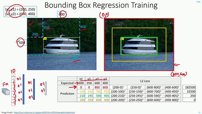
객체 탐지를 위한 바운딩 박스 회귀를 실시하기 위해서 우리는 신경망 구조를 조금 변경해야 합니다:
**이 글의 핵심**
- 신경망의 출력 부분(head of the network)에 바운딩 박스의 좌측 상단 및 우측 하단의 좌표(x, y)에 해당하는 4개의 뉴런 노드가 있는 완전연결층을 연결합니다.
- 4개의 뉴런 노드에 대해서 sigmoid 활성화 함수를 구현하여 출력의 범위가 [0, 1] 사이가 되도록 합니다.
- mse 혹은 mae 손실 함수를 이용하여 모델을 훈련 데이터에 대해서 학습시킵니다. 훈련 데이터는 (1) 입력 이미지와 (2) 이미지 내 객체의 바운딩 박스에 대한 정보가 있어야 합니다.
훈련을 마치면 우리의 신경망은 객체에 대한 바운딩 박스를 예측할 수 있을 겁니다.
이 튜토리얼에서는 한 개의 클래스에 대해서만 객체 탐지를 하도록 하겠지만 이후에 다른 글에서 다중 클래스에 대한 객체 탐지를 다루도록 할게요.
데이터셋
<요약> CALTECH-101 데이터셋 일부: 800개 비행기 이미지 + 바운딩 박스 좌표 레이블
이 튜토리얼에서 사용할 예시 데이터셋은 CALTECH-101 데이터셋의 일부이다. 이 데이터를 통해 우리의 객체 탐지 모델을 훈련시켜보도록 하자.
구체적으로, 우리는 airplane 클래스에 해당하는 800개의 이미지와 이미지 내 비행기가 있는 위치를 알려주는 바운딩박스 좌표를 데이터셋으로 쓸 것이다. <그림 2>를 참고하도록 하자.
우리의 목표는 이미지 내에 비행기가 어디 있는지 정확하게 예측할 수 있는 객체 탐지 모델을 훈련시키는 것이다.

원본 데이터셋 링크: Caltech101
Caltech101
We have collected a new data-set of 256 object categories!! *** New Expanded / Improved Caltech 256 Category Data-Set *** Click Here to access the New Data-Set: Caltech256 ---> Description Pictures of objects belonging to 101 categories. About 40 to 800 im
www.vision.caltech.edu
소스코드
파일구조
파일구조는 다음과 같이 설정하자. 앞서 언급한대로, 이번 튜토리얼에서는 데이터셋으로 비행기 800개 사진과 그에 대응하는 바운딩 박스 좌표가 들어있는 csv 파일을 사용하도록 하겠다.

이 튜토리얼에서 검토해볼 파이썬 파일은 다음과 같다:
- config.py : 변수명 등 환경을 설정해줄 파일
- train.py : 훈련시키는 코드. 데이터를 로드하고 VGG-16 백본 모델을 우리 데이터에 미세조정해줄 것이다. 훈련 결과로 출력되는 결과물(모델, 훈련 경과표, 테스트 이미지 목록)은 output/ 아래 경로에 저장될 것이다.
- predict.py : 데모 코드. 이미지를 로드하고 테스트 이미지에 바운딩 박스를 예측한다.
가장 먼저 살펴볼 코드는 config.py이다.
config.py
바운딩 박스 회귀를 학습할 코드를 구현하기 전에 먼저 간단하게 계속해서 사용할 변수명과 경로를 설정해주는 코드를 짜보자.
# import the necessary packages
import os

# define the base path to the input dataset and then use it to derive
# the path to the images directory and annotation CSV file
BASE_PATH = "dataset"
IMAGES_PATH = os.path.sep.join([BASE_PATH, "images"])
ANNOTS_PATH = os.path.sep.join([BASE_PATH, "airplanes.csv"])

# define the path to the base output directory
BASE_OUTPUT = "output"

# define the path to the output serialized model, model training plot,
# and testing image filenames
MODEL_PATH = os.path.sep.join([BASE_OUTPUT, "detector.h5"])
PLOT_PATH = os.path.sep.join([BASE_OUTPUT, "plot.png"])
TEST_FILENAMES = os.path.sep.join([BASE_OUTPUT, "test_images.txt"])

# initialize our initial learning rate, number of epochs to train
# for, and the batch size
INIT_LR = 1e-4
NUM_EPOCHS = 25
BATCH_SIZE = 32
train.py
이 훈련 코드는,
- 데이터셋을 로드하고
- 완전연결층을 제거한 VGG16 모델을 불러와 우리가 원하는 완전연결층을 넣고 (최종 레이어에 노드 4개)
- 데이터셋에 맞게 사전훈련된 모델을 미세조정한다.
바운딩 박스 회귀를 이해하는 가장 쉬운 방법은 코드를 통해 보는 것이다. 바로 코드를 보도록 해보자!
# import the necessary packages
from pyimagesearch import config
from tensorflow.keras.applications import VGG16
from tensorflow.keras.layers import Flatten
from tensorflow.keras.layers import Dense
from tensorflow.keras.layers import Input
from tensorflow.keras.models import Model
from tensorflow.keras.optimizers import Adam
from tensorflow.keras.preprocessing.image import img_to_array
from tensorflow.keras.preprocessing.image import load_img
from sklearn.model_selection import train_test_split
import matplotlib.pyplot as plt
import numpy as np
import cv2
import os

# load the contents of the CSV annotations file
print("[INFO] loading dataset...")
rows = open(config.ANNOTS_PATH).read().strip().split("\n")

# initialize the list of data (images), our target output predictions
# (bounding box coordinates), along with the filenames of the
# individual images
data = []
targets = []
filenames = []

# loop over the rows
for row in rows:
	# break the row into the filename and bounding box coordinates
	row = row.split(",")
	(filename, startX, startY, endX, endY) = row
필요한 라이브러리를 가져오고, 훈련 데이터를 로드하자.
참고로 훈련 데이터에 대한 레이블링 csv 파일은 아래 그림과 같이 되어있다.

다음으로, 이미지의 경로를 통해 cv2를 이용해 각각 불러옵니다. 이미지의 높이와 너비를 h, w라는 변수에 저장한 후 바운딩 박스를 해당 이미지의 높이 및 너비로 나눠줌으로써 [0, 1] 사이의 값으로 스케일링해줍니다.
또한 load_img 메소드를 활용해서 cv2로 로드한 이미지를 덮어씌우고, VGG16의 입력으로 들어갈 수 있도록 사이즈를 224 x 224로 조정해주고 넘파이 형식으로 바꿔줍니다. 그리고 반복문 이전에 미리 준비한 변수 리스트에 해당 값을 담아줍니다.
	# derive the path to the input image, load the image (in OpenCV
	# format), and grab its dimensions
	imagePath = os.path.sep.join([config.IMAGES_PATH, filename])
	image = cv2.imread(imagePath)
	(h, w) = image.shape[:2]

	# scale the bounding box coordinates relative to the spatial
	# dimensions of the input image
	startX = float(startX) / w
	startY = float(startY) / h
	endX = float(endX) / w
	endY = float(endY) / h

    # load the image and preprocess it
	image = load_img(imagePath, target_size=(224, 224))
	image = img_to_array(image)

	# update our list of data, targets, and filenames
	data.append(image)
	targets.append((startX, startY, endX, endY))
	filenames.append(filename)
위 과정을 거치면 데이터 로드는 완료된 겁니다.
이제 각종 전처리 작업을 해보도록 하죠. 먼저 정규화를 통해 각 픽셀 값을 [0, 1] 사이의 값으로 만들어줍니다. 그리고 훈련셋과 테스트셋으로 분리하도록 해요.
# convert the data and targets to NumPy arrays, scaling the input
# pixel intensities from the range [0, 255] to [0, 1]
data = np.array(data, dtype="float32") / 255.0
targets = np.array(targets, dtype="float32")

# partition the data into training and testing splits using 90% of
# the data for training and the remaining 10% for testing
split = train_test_split(data, targets, filenames, test_size=0.10,
	random_state=42)

# unpack the data split
(trainImages, testImages) = split[:2]
(trainTargets, testTargets) = split[2:4]
(trainFilenames, testFilenames) = split[4:]

# write the testing filenames to disk so that we can use them
# when evaluating/testing our bounding box regressor
print("[INFO] saving testing filenames...")
f = open(config.TEST_FILENAMES, "w")
f.write("\n".join(testFilenames))
f.close()
이제 모델을 준비해봐요.
미세조정은 다음과 같은 절차로 수행되요:
- VGG16 모델을 로드하는데, 그 가중치는 ImageNet에 사전훈련된 것(weights='imagenet')이고, 완전연결층이 없는 것(include_top=False)이어야 해요.
- VGG16 신경망 내에 있는 모든 레이어의 가중치를 동결시켜요(freeze).
- 그리고 CNN에서 이어지는 DNN을 연결시키도록 해요. 이 완전연결층은 바운딩 박스의 좌표에 대응되도록 마지막 레이어의 노드는 4개로 설정해요.
- 마지막으로 모델의 입력층과 출력층을 정해주면서 마무리하도록 해요.
# load the VGG16 network, ensuring the head FC layers are left off
vgg = VGG16(weights="imagenet", include_top=False,
	input_tensor=Input(shape=(224, 224, 3)))

# freeze all VGG layers so they will *not* be updated during the
# training process
vgg.trainable = False

# flatten the max-pooling output of VGG
flatten = vgg.output
flatten = Flatten()(flatten)

# construct a fully-connected layer header to output the predicted
# bounding box coordinates
bboxHead = Dense(128, activation="relu")(flatten)
bboxHead = Dense(64, activation="relu")(bboxHead)
bboxHead = Dense(32, activation="relu")(bboxHead)
bboxHead = Dense(4, activation="sigmoid")(bboxHead)

# construct the model we will fine-tune for bounding box regression
model = Model(inputs=vgg.input, outputs=bboxHead)
모델을 준비시켰으니 이제 훈련을 해봐요.
컴파일은 Adam 옵티마이저로, loss 함수는 mse로 설정해요.
훈련할 때 검증은 데이터 로드할 때 분리한 테스트셋으로 해요.
마지막으로 모델 저장 및 학습표를 시각화하고 저장하도록 해요.
# initialize the optimizer, compile the model, and show the model
# summary
opt = Adam(lr=config.INIT_LR)
model.compile(loss="mse", optimizer=opt)
print(model.summary())

# train the network for bounding box regression
print("[INFO] training bounding box regressor...")
H = model.fit(
	trainImages, trainTargets,
	validation_data=(testImages, testTargets),
	batch_size=config.BATCH_SIZE,
	epochs=config.NUM_EPOCHS,
	verbose=1)

# serialize the model to disk
print("[INFO] saving object detector model...")
model.save(config.MODEL_PATH, save_format="h5")

# plot the model training history
N = config.NUM_EPOCHS
plt.style.use("ggplot")
plt.figure()
plt.plot(np.arange(0, N), H.history["loss"], label="train_loss")
plt.plot(np.arange(0, N), H.history["val_loss"], label="val_loss")
plt.title("Bounding Box Regression Loss on Training Set")
plt.xlabel("Epoch #")
plt.ylabel("Loss")
plt.legend(loc="lower left")
plt.savefig(config.PLOT_PATH)
터미널에서 파일 실행하기↓
$ python train.py
[INFO] loading dataset...
[INFO] saving testing filenames...
훈련이 끝나면 output 경로 아래에 (1) detector.h5, (2) plot.png, (3) test_images.txt 파일들이 만들어질 겁니다.
predict.py
# import the necessary packages
from pyimagesearch import config
from tensorflow.keras.preprocessing.image import img_to_array
from tensorflow.keras.preprocessing.image import load_img
from tensorflow.keras.models import load_model
import numpy as np
import mimetypes
import argparse
import imutils
import cv2
import os

# construct the argument parser and parse the arguments
ap = argparse.ArgumentParser()
ap.add_argument("-i", "--input", required=True,
	help="path to input image/text file of image filenames")
args = vars(ap.parse_args())

# determine the input file type, but assume that we're working with
# single input image
filetype = mimetypes.guess_type(args["input"])[0]
imagePaths = [args["input"]]

# if the file type is a text file, then we need to process *multiple*
# images
if "text/plain" == filetype:
	# load the filenames in our testing file and initialize our list
	# of image paths
	filenames = open(args["input"]).read().strip().split("\n")
	imagePaths = []

	# loop over the filenames
	for f in filenames:
		# construct the full path to the image filename and then
		# update our image paths list
		p = os.path.sep.join([config.IMAGES_PATH, f])
		imagePaths.append(p)

# load our trained bounding box regressor from disk
print("[INFO] loading object detector...")
model = load_model(config.MODEL_PATH)

# loop over the images that we'll be testing using our bounding box
# regression model
for imagePath in imagePaths:
	# load the input image (in Keras format) from disk and preprocess
	# it, scaling the pixel intensities to the range [0, 1]
	image = load_img(imagePath, target_size=(224, 224))
	image = img_to_array(image) / 255.0
	image = np.expand_dims(image, axis=0)

	# make bounding box predictions on the input image
	preds = model.predict(image)[0]
	(startX, startY, endX, endY) = preds

	# load the input image (in OpenCV format), resize it such that it
	# fits on our screen, and grab its dimensions
	image = cv2.imread(imagePath)
	image = imutils.resize(image, width=600)
	(h, w) = image.shape[:2]

	# scale the predicted bounding box coordinates based on the image
	# dimensions
	startX = int(startX * w)
	startY = int(startY * h)
	endX = int(endX * w)
	endY = int(endY * h)

	# draw the predicted bounding box on the image
	cv2.rectangle(image, (startX, startY), (endX, endY),
		(0, 255, 0), 2)

	# show the output image
	cv2.imshow("Output", image)
	cv2.waitKey(0)
터미널에서 파일 실행하기↓
$ python predict.py --input dataset/images/image_0697.jpg
[INFO] loading object detector...

$ python predict.py --input output/test_images.txt
[INFO] loading object detector...
한계점
축하합니다! 성공적으로 바운딩 박스 회귀 모델을 훈련시켰네요! 하지만, 이 구조의 한계점은 오직 한 개의 클래스에 대한 바운딩 박스만 예측할 수 있다는 점입니다.
만약에 우리가 다수의 클래스에 해당하는 객체들을 탐지하려고 하면 어떡하죠? "비행기"뿐만 아니라 "오토바이", "자동차", "트럭" 또한 탐지하고 싶다면요?
다중 클래스 객체 탐지에 대해서 바운딩 박스를 그리는 건 가능하기나 할까요?
정답은 '가능하다'입니다. 해당 내용은 다음 튜토리얼에서 다루도록 할게요. 힌트는 CNN 모델에서 가지를 두 가지로 치는 거랍니다. 다음 튜토리얼에서 봐요~
PyImageSearch University Courses: You can master Computer Vision, Deep Learning, and OpenCV
'Coding > Image' 카테고리의 다른 글
| [6] Multi-class Object Detection (0) | 2021.05.07 |
|---|---|
| SSD (0) | 2021.05.07 |
| Morphological Transformations (0) | 2021.05.07 |
| Instance Segmentation + Mask RCNN (0) | 2021.05.07 |
| Image hashing (0) | 2021.05.07 |


